Kaggle COVID-19 CT 이미지의 분류를 딥러닝으로 수행한 프로젝트로 CNN 기반으로 코로나 감염 여부를 분류하는 것이 목적입니다. 앞의 포스팅에 이어 적은 내용입니다.
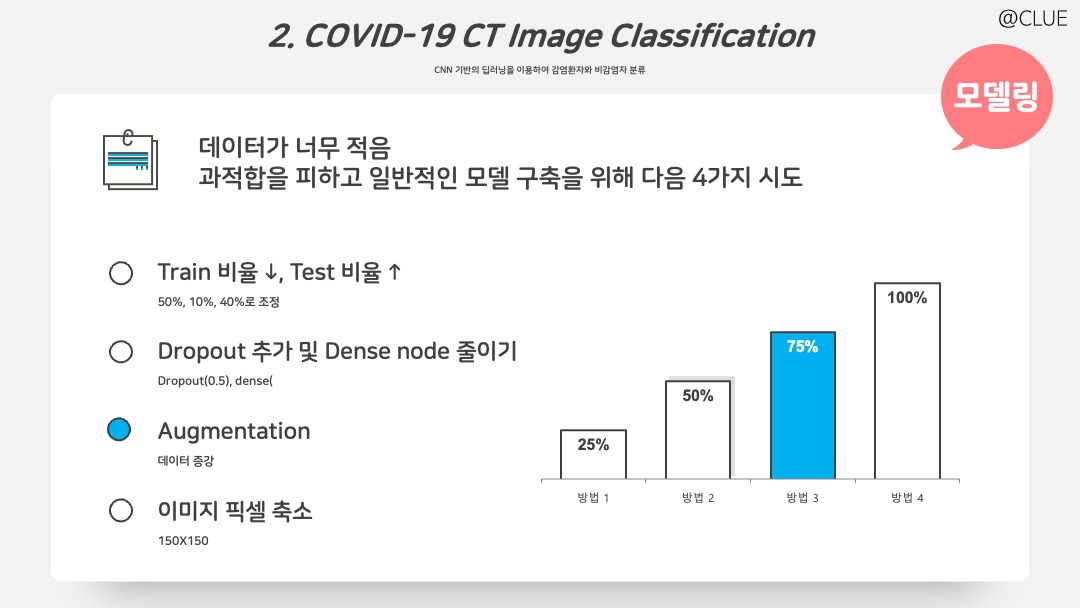
앞 포스팅 CNN 결과 정확도는 높은 편이나, 원 데이터가 딥러닝 모델을 돌리기에 너무 적기 때문에 과적합을 피하고 general한 모델 구축을 위해 네 가지를 시도한다. 1. Train/Validate/Test 비율을 50%/10%/40%로 변경하여 Train 비율을 낮추고 Test 비율을 늘린다. 2. Dropout 추가 및 Dense Node 줄인다. 3. 데이터를 증강한다. 4. 이미지 픽셀을 더 작게 150*150으로 축소한다.
# 1. 비율 변경은 앞 포스팅을 참고해서 변형하면 된다.

# 3. Train 데이터를 증강한다.
train_datagen = ImageDataGenerator(
    rescale = 1./255,
    rotation_range = 40,
    width_shift_range = 0.2,
    height_shift_range = 0.2,
    shear_range = 0.2,
    zoom_range=0.2,
    horizontal_flip = True,
    fill_mode = 'nearest'
)

vali_datagen = ImageDataGenerator(rescale=1./255)
test_datagen = ImageDataGenerator(rescale=1./255)

train_generator = train_datagen.flow_from_directory(
    train_dir,
    target_size = (150, 150),
    batch_size = 30,
    class_mode = 'binary',
    color_mode='grayscale'
)

validation_generator = vali_datagen.flow_from_directory(
    vali_dir,
    target_size = (150, 150),
    batch_size = 30,
    class_mode = 'binary',
    color_mode='grayscale'
)

test_generator = test_datagen.flow_from_directory(
    test_dir,
    target_size = (150, 150),
    batch_size = 30,
    class_mode = 'binary',
    color_mode='grayscale'
)

# 2. Dropout 추가 및 Dense Node를 줄인다. & 4. 이미지 픽셀을 더 작게 150*150으로 축소한다.
IMAGE_ROWS = 150
IMAGE_COLS = 150
BATCH_SIZE = 30
IMAGE_SHAPE = (IMAGE_ROWS,IMAGE_COLS,1)

import tensorflow as tf
from tensorflow.keras import layers
from tensorflow.keras import models

model2 = models.Sequential()
model2.add(layers.Conv2D(32, (3,3), activation='relu', input_shape=IMAGE_SHAPE))
model2.add(layers.MaxPooling2D((2,2)))
model2.add(layers.Dropout(0.5))
model2.add(layers.Conv2D(64, (3,3), activation='relu'))
model2.add(layers.MaxPooling2D((2,2)))
model2.add(layers.Flatten())
model2.add(layers.Dropout(0.5))
model2.add(layers.Dense(64, activation='relu'))
model2.add(layers.Dense(1, activation='sigmoid'))

model2.summary()

from tensorflow.keras import optimizers

model2.compile(optimizer=optimizers.Adam(learning_rate=1e-4), # 'rmsprop',
               loss='binary_crossentropy',
               metrics=['acc'])

history2 = model2.fit_generator(train_generator, steps_per_epoch=15, epochs=10, validation_data = validation_generator, validation_steps = 1)

# 결과 및 시각화 코드는 앞 포스팅 참고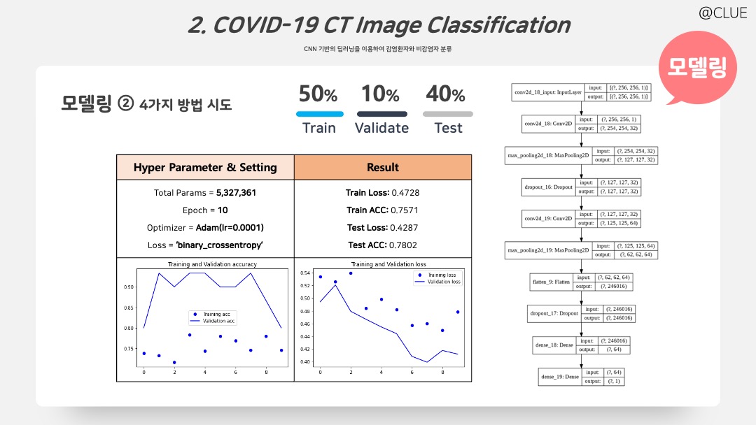
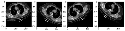
위는 모델링 결과이다. 참고로 증강하고 픽셀을 낮춘 데이터의 예시는 아래와 같다.
# 증강 데이터 확인
import os
from tensorflow.keras.preprocessing import image

train_dir = '/content/gdrive/My Drive/COVID_CT_NEW/train'
one_fname = os.path.join(str(train_dir + '/Infected/202.jpg'))
img = image.load_img(one_fname, target_size=(258,258))

x = image.img_to_array(img)
x = x.reshape((1,)+x.shape)

i = 0
plt.figure(figsize=(12,6))

for batch in train_datagen.flow(x, batch_size=1):
    plt.subplot(1, 4,i+1)
    plt.imshow(image.array_to_img(batch[0]))

    i += 1
    if i % 4 == 0:
        break

plt.show()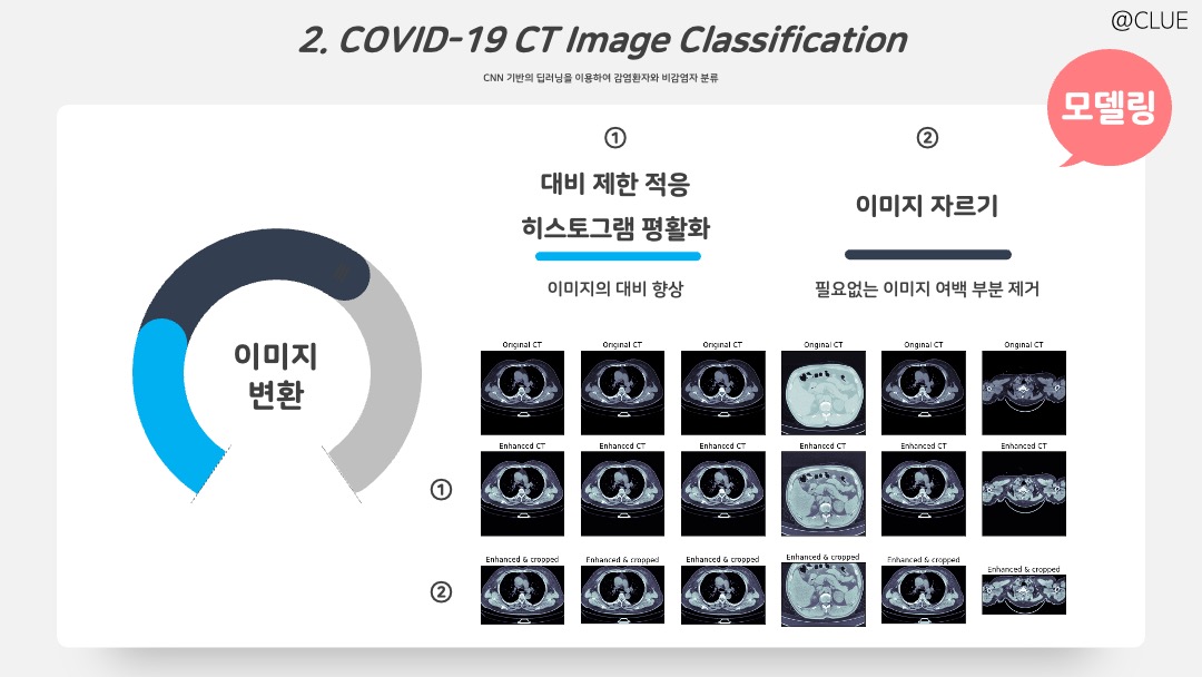
위의 결과를 확인해본 결과를 Accuracy가 많이 감소하게 되고, Test Accuracy로 0.78이 출력되었다. 여기서부터 이제 이미지를 변형하여 더욱 성능을 높이고, 효율적인 모델 구축을 시도하기 위해 두 가지를 시도했다.
- 대비 제한 적응 히스토그램 평활화(CLAHE): 이미지에서 대비를 향상시키기 위해 사용하는 방법이다. 이를 수행하면 다음과 같이 이미지의 대비가 조금 더 선명해진다.
- 이미지 자르기: 이미지에서 필요하지 않은 여백을 자르면 굳이 합성곱 필터를 거치지 않아도 되기 때문에 파라미터 수를 줄이고 특징을 더 잘 잡아내도록 도움이 될 수 있다. 이를 수행하면 3번째 행 이미지와 같이 이미지의 검은 여백 부분이 잘린다.
# 1. 대비 제한 적응 히스토그램 평활화(CLAHE)
clahe = cv2.createCLAHE(clipLimit=3.0)
def clahe_enhancer(img, clahe, axes):
    img = np.uint8(img*255)
    clahe_img = clahe.apply(img)

    if len(axes) > 0 :
        axes[0].imshow(img, cmap='bone')
        axes[0].set_title("Original CT scan")
        axes[0].set_xticks([]); axes[0].set_yticks([])

        axes[1].imshow(clahe_img, cmap='bone')
        axes[1].set_title("CLAHE Enhanced CT scan")
        axes[1].set_xticks([]); axes[1].set_yticks([])

        if len(axes) > 2 :
            axes[2].hist(img.flatten(), alpha=0.4, label='Original CT scan')
            axes[2].hist(clahe_img.flatten(), alpha=0.4, label="CLAHE Enhanced CT scan")
            plt.legend()

    return(clahe_img)

# 이미지 확인 코드
fig, axes = plt.subplots(3, 6, figsize=(18,8))
img_size = 512

for ii in range(0,6):
    img = cv2.resize(infected_[ii], dsize=(img_size, img_size), interpolation=cv2.INTER_AREA)
    xmax, xmin = img.max(), img.min()
    img = (img - xmin)/(xmax - xmin)
    clahe_img = clahe_enhancer(img, clahe, list(axes[:, ii]))

# 2. 이미지 자르기
def get_contours(img):
    img = np.uint8(img*255)

    kernel = np.ones((3,3),np.float32)/9
    img = cv2.filter2D(img, -1, kernel)

    ret, thresh = cv2.threshold(img, 50, 255, cv2.THRESH_BINARY)
    contours, hierarchy = cv2.findContours(thresh, 2, 1)
    #Areas = [cv.contourArea(cc) for cc in contours]; print(Areas)

    size = get_size(img)
    contours = [cc for cc in contours if contourOK(cc, size)]
    return contours

def get_size(img):
    ih, iw = img.shape
    return iw * ih

def contourOK(cc, size):
    x, y, w, h = cv2.boundingRect(cc)
    if ((w < 50 and h > 150) or (w > 150 and h < 50)) :
        return False # too narrow or wide is bad
    area = cv2.contourArea(cc)
    return area < (size * 0.5) and area > 200

def find_boundaries(img, contours):
    ih, iw = img.shape
    minx = iw
    miny = ih
    maxx = 0
    maxy = 0

    for cc in contours:
        x, y, w, h = cv2.boundingRect(cc)
        if x < minx: minx = x
        if y < miny: miny = y
        if x + w > maxx: maxx = x + w
        if y + h > maxy: maxy = y + h

    return (minx, miny, maxx, maxy)

def crop_(img, boundaries):
    minx, miny, maxx, maxy = boundaries
    return img[miny:maxy, minx:maxx]

def crop_img(img, axes) :
    contours = get_contours(img)
    #plt.figure() # uncomment to troubleshoot
    #canvas = np.zeros_like(img)
    #cv.drawContours(canvas , contours, -1, (255, 255, 0), 1)
    #plt.imshow(canvas)
    bounds = find_boundaries(img, contours)
    cropped_img = crop_(img, bounds)

    if len(axes) > 0 :
        axes[0].imshow(img, cmap='bone')
        axes[0].set_title("Original CT scan")
        axes[0].set_xticks([]); axes[0].set_yticks([])

        axes[1].imshow(cropped_img, cmap='bone')
        axes[1].set_title("Cropped CT scan")
        axes[1].set_xticks([]); axes[1].set_yticks([])

    return cropped_img, bounds

fig, axes = plt.subplots(3, 6, figsize=(18,9))

for ii in range(0,6):
    img = cv2.resize(infected_[ii], dsize=(img_size, img_size), interpolation=cv2.INTER_AREA)
    xmax, xmin = img.max(), img.min()
    img = (img - xmin)/(xmax - xmin)
    _, bounds = crop_img(img, [])
    axes[0,ii].imshow(img, cmap='bone')
    axes[0,ii].set_title('Original CT')
    axes[0,ii].set_xticks([]); axes[0,ii].set_yticks([])

    clahe_img = clahe_enhancer(img, clahe, [])
    axes[1,ii].imshow(clahe_img, cmap='bone')
    axes[1,ii].set_title('Enhanced CT')
    axes[1,ii].set_xticks([]); axes[1,ii].set_yticks([])

    cropped_img = crop_(clahe_img, bounds)
    axes[2,ii].imshow(cropped_img, cmap='bone')
    axes[2,ii].set_title('Enhanced & cropped')
    axes[2,ii].set_xticks([]); axes[2,ii].set_yticks([])

# 전체에 적용, clahe, crop (기본 이미지 512X512에 먼저 적용)
infected_f = []

for ii in range(infected_.shape[0]):
    img_ct = cv2.resize(infected_[ii], dsize=(img_size, img_size),
                        interpolation=cv2.INTER_AREA)
    xmax, xmin = img_ct.max(), img_ct.min()
    img_ct = (img_ct - xmin)/(xmax - xmin)
    clahe_ct = clahe_enhancer(img_ct, clahe, [])
    cropped_ct = crop_(clahe_ct, bounds)
    infected_f.append(cropped_ct)

# 전체에 적용, clahe, crop (기본 이미지 512X512에 먼저 적용)
n_infected_f = []

for ii in range(n_infected_.shape[0]):
    img_ct = cv2.resize(n_infected_[ii], dsize=(img_size, img_size),
                        interpolation=cv2.INTER_AREA)
    xmax, xmin = img_ct.max(), img_ct.min()
    img_ct = (img_ct - xmin)/(xmax - xmin)
    clahe_ct = clahe_enhancer(img_ct, clahe, [])
    cropped_ct = crop_(clahe_ct, bounds)
    n_infected_f.append(cropped_ct)

# resize and reshape
num_pix = 512
del_lst = []
for ii in tqdm.tqdm(range(len(infected_f))) :
    try :
        infected_f[ii] = cv2.resize(infected_f[ii], dsize=(num_pix, num_pix), interpolation=cv2.INTER_AREA)
        infected_f[ii] = np.reshape(infected_f[ii], (num_pix, num_pix, 1))
    except :
        del_lst.append(ii)

for idx in del_lst[::-1] :
    del infected_f[idx]

# resize and reshape
num_pix = 512
del_lst = []
for ii in tqdm.tqdm(range(len(n_infected_f))) :
    try :
        n_infected_f[ii] = cv2.resize(n_infected_f[ii], dsize=(num_pix, num_pix), interpolation=cv2.INTER_AREA)
        n_infected_f[ii] = np.reshape(n_infected_f[ii], (num_pix, num_pix, 1))
    except :
        del_lst.append(ii)

for idx in del_lst[::-1] :
    del n_infected_f[idx]

# 비감염자 0번째 이미지 확인
plt.figure()

plt.imshow(infected_f[0][:,:,0], cmap='bone') # 0번째
plt.title("Enhanced & Cropped CT")

# 앞의 포스팅을 참고하여 이렇게 변형된 데이터들을 다시 폴더에 나눠 저장해서 데이터 증강을 한다. (앞의 1-4. 과정 또한 이후 그대로 수행)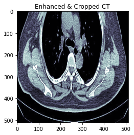
변형된 이미지는 위와 같다.
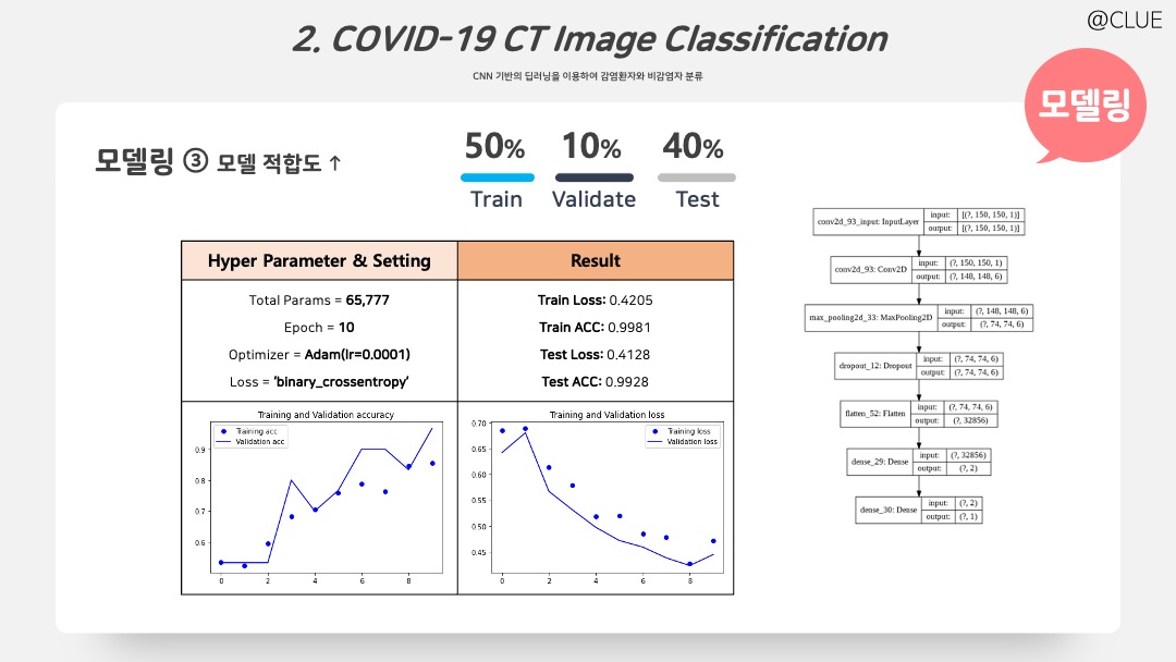
변형된 이미지를 이용하여 앞의 모델보다 더 간단한 모델을 적합한 결과이다. 처음 모델 파라미터 개수의 0.2%에 해당하는 개수만으로도 충분히 높은 Accuracy를 얻을 수 있다.
# ImageGenerator 코트 생략, 위를 참조

IMAGE_ROWS = 150
IMAGE_COLS = 150
BATCH_SIZE = 30
IMAGE_SHAPE = (IMAGE_ROWS,IMAGE_COLS,1)

import tensorflow as tf
from tensorflow.keras import layers
from tensorflow.keras import models

model4 = models.Sequential()
model4.add(layers.Conv2D(6, (3,3), activation='relu', input_shape=IMAGE_SHAPE))
model4.add(layers.MaxPooling2D((2,2)))
model4.add(layers.Dropout(0.8))
# model4.add(layers.Conv2D(64, (3,3), activation='relu'))
# model4.add(layers.MaxPooling2D((2,2)))
model4.add(layers.Flatten())
# model4.add(layers.Dropout(0.5))
model4.add(layers.Dense(2, activation='relu'))
model4.add(layers.Dense(1, activation='sigmoid'))

model4.summary()

from tensorflow.keras import optimizers

model4.compile(optimizer=optimizers.Adam(learning_rate=1e-4), # 'rmsprop',
               loss='binary_crossentropy',
               metrics=['acc'])

history4 = model4.fit_generator(train_generator, steps_per_epoch=15, epochs=10, validation_data = validation_generator, validation_steps = 1)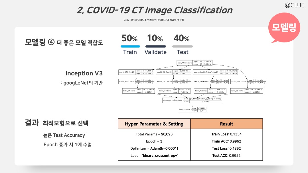
마지막으로 Test Accuracy를 조금 더 향상시키기 위해 Reduced Inception V3 모델을 시도했다. Inception V3는 구글넷에 기반이 되는 모델이기도 하하며 구조는 위와 같다. 3번의 반복으로도 앞의 모델보다 Test Accuracy에 향상이 나타나고, 그 이상 반복하면 Validation Accuracy는 1에 수렴한다. X-ray classification에서도 사용되는 모델이며, 흑백 이미지 분류에 많이 사용한다. 파라미터도 앞의 모델에 비해 많이 증가하지 않아 해당 모델을 최적 모형으로 선택한다.
def inception_block_dim_reduce(input_layer, filter1, filter2, filter3, reduce1, reduce2, pool_proj, activation='relu', pull=False):
    conv1x1 = Conv2D(filter1, kernel_size=(1,1), padding='same', activation=activation)(input_layer)
    conv3x3_reduce = Conv2D(reduce1, kernel_size=(1,1), padding='same', activation=activation)(input_layer)
    conv3x3 = Conv2D(filter2, kernel_size=(3,3), padding='same', activation=activation)(conv3x3_reduce)
    conv5x5_reduce = Conv2D(reduce2, kernel_size=(1,1), padding='same', activation=activation)(input_layer)
    conv5x5 = Conv2D(filter3, kernel_size=(5,5), padding='same', activation=activation)(conv5x5_reduce)
    pooling = MaxPooling2D((3,3), strides=(1,1), padding='same')(input_layer)
    pool_proj = Conv2D(pool_proj, kernel_size=(1,1), padding='same', activation=activation)(pooling)
    output_layer = concatenate([conv1x1, conv3x3, conv5x5, pool_proj])

    # Googlenet exracts pool_proj in order to ensemble in three cases
    if pull == True:
        return output_layer, pool_proj

    return output_layer

shape = (224,224,3)


from tensorflow.keras.layers import Conv2D, MaxPooling2D, AveragePooling2D, concatenate, Input, Dense, Flatten
from tensorflow.keras import models

inputs = Input(IMAGE_SHAPE)
conv1x1 = Conv2D(1, kernel_size=(7,7), padding='same', activation='relu')(inputs)
conv3x3_reduce = Conv2D(1, kernel_size=(1,1), padding='same', activation='relu')(inputs)
conv3x3 = Conv2D(1, kernel_size=(3,3), padding='same', activation='relu')(conv3x3_reduce)
conv5x5_reduce = Conv2D(1, kernel_size=(1,1), padding='same', activation='relu')(inputs)
conv5x5 = Conv2D(1, kernel_size=(5,5), padding='same', activation='relu')(conv5x5_reduce)
pooling = MaxPooling2D((4,4), strides=(1,1), padding='same')(inputs)
pool_proj = Conv2D(1, kernel_size=(1,1), padding='same', activation='relu')(pooling)

conv1x1_out = Flatten()(conv1x1)
conv3x3_out = Flatten()(conv3x3)
conv5x5_out = Flatten()(conv5x5)
pooling_out = Flatten()(pool_proj)

concat = concatenate([conv1x1_out, conv3x3_out, conv5x5_out, pooling_out])
output_layer = Dense(1, activation='sigmoid')(concat)

model6 = models.Model(inputs, output_layer)

from tensorflow.keras import optimizers

model6.compile(optimizer=optimizers.Adam(learning_rate=1e-4), # 'rmsprop',
               loss='binary_crossentropy',
               metrics=['acc'])

history6 = model6.fit_generator(train_generator, steps_per_epoch=15, epochs=3, validation_data = validation_generator, validation_steps = 1)
# epoch 세 번으로도 충분함

# 모델 구조 확인
from tensorflow.keras.utils import plot_model

plot_model(model6, to_file='CNN6.png', show_shapes=True)
특히 Reduced Inception V3를 이용하여 Convolution1x1 레이어를 이용하여 dimension을 줄여, AlexNet보다 12배만큼 적은 파라미터로 훈련하게 된다. 이를 최적 모형으로 선정했다.
피피티 디자인 저작권은 @PPTBIZCAM